Gaussian Process Prediction

GP Regression on Hand-Drawn Trajectories

Gaussian Process (GP) Regression is a powerful tool for performing inference on sparse data, such as in situations where the whole trajectory cannot be observed or it is impractical to do so. For example, if we are trying to quantify the mineral content in a spatial field- where only a finite number of samples are to be collected- then the values at unknown locations can be predicted using a closely-related method known as kriging. Consider being given a data set which cointains a few points along a trajectory, and the goal is to infer what the whole trajectory looks like. If you have prior knowledge on the behavior of the function in between regression points, a covariance function (kernel) can be chosen, acting as a prior on the distribution of functions that the true process is sampled from (although choosing a kernel is not always straightforward). Upon observing new data points, conditional inference allows for combining the existing (prior) estimate and the newly observed data to obtain a new (posterior) estimate of the underlying function. This iterative procedure is convenient for updating our belief of the true trajectory as data comes sequentially, but often the conditional inference step only needs to be applied once (in the event where all of the data points are provided at once, as in the upcoming example).

GP Regression is a compelling option for nonlinear regression since it can be used to quantify the uncertainty of values in between observed points (with credible bands) and provides a flexible way to incorporate a prior with covariance functions. Moreover, the kernel hyperparameters can be estimated by maximizing the marginal likelihood of the training points given their domain locations, and this post will describe the process for doing so. With the popularity of neural networks, an obvious question is whether a neural network can be used for the prediction instead. I did a project on this with a peer, where both methods were used to predict a hand-drawn trajectory of the letter e, and both methods predicted the full trajectory well. I’m not an expert in this area, but I wouldn’t be surprised if there are good ways to approximate the credible bands using NNs (e.g., with stochastic forward passes), but that’s beyond the scope of this post. Overall, there are some cool features in GP Regression that a vanilla, feed-forward NN does not provide out of the box. Let’s check it out!

The Hand-Drawn Data Set

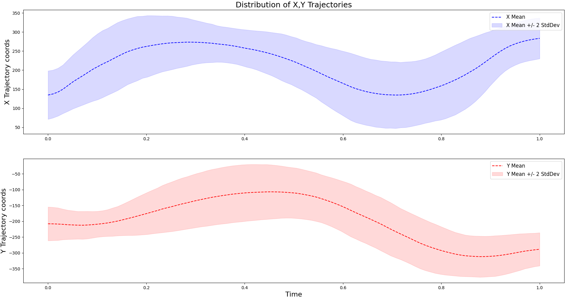
The following data set (left) was created using a computer mouse and python script to record the cursor positions on the canvas from drawing the letter e. All demonstrations are resampled to have the same length. These trajectories can be used by extracting the \(x\) and \(y\) dimensions to fit two Gaussian Processes independently.
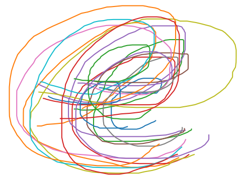
Distribution of hand-drawn letter e's
Distribution of X (top) and Y (bottom) Coordinates from start to finish (not standardized)

Choosing the Kernel

As noted above, different kernels can be chosen based on the data points observed in the sample set. Looking at the trajectories for the \(X\) and \(Y\) components of the letter e, we can see that they exhibits smooth (almost sinusoidal) behavior. Knowing this, the Squared Exponential (SE) kernel becomes a good candidate since it is often used for fitting smooth functions. Other popular kernels for fitting Gaussian Processes include the Rational Quadratic (RQ) and Matern kernel, which is grounded with many theoretical properties. We will use all three of these kernels and compare their marginal likelihoods to determine which one to use. The respective definitions for these kernels are listed below.

$$ k(x_i, x_j) = \sigma_f^2 \exp{ \left( -\frac{(x_i- x_j)^2}{2\ell^2} \right)} $$
Squared Exponential Kernel
$$ k(x_i, x_j) = \sigma_f^2 \left( 1 + \frac{(x_i - x_j)^2}{2 \alpha \ell^2} \right)^{-\alpha} $$
Rational Quadratic Kernel
$$ k(x_i, x_j) = \frac{2^{1-\nu}}{\Gamma(\nu)}\Bigg( \frac{\sqrt{2\nu} \lVert x_i - x_j \rVert }{\ell} \Bigg)^\nu K_\nu\Bigg( \frac{\sqrt{2\nu} \lVert x_i - x_j \rVert }{\ell} \Bigg) $$
Matern Kernel

The following code implements the kernels above by inheriting from a Kernel base class (see Appendix), and the mathematical defintions are specified in the cov method. Included in each class are the respective kernel hyperparameters which later optimized. The Kernel instance is passed to the Gaussian Process class for prediction in the upcoming section. The cdist function from scipy is a computationally efficient way to compute the distance between pairs of points compared to naive \(O(n^2)\) implementation using for loops. For more information on kernels, check out the references and The Kernel Cookbook 1.

from scipy.spatial.distance import cdist
from scipy.special import gamma, kv

EPSILON = 1e-8

# Define the SE Kernel
class SquaredExponential(Kernel):
    def __init__(self, sigma_f: Hyperparam = None, lengthscale: Hyperparam = None):
        _hyperparams = {
            'sigma_f' : sigma_f,
            'lengthscale' : lengthscale,
        }
        super().__init__(_hyperparams)

    # Covariance function definition
    def cov(self, xi, xj):
        sf, l = self.hyperparams['sigma_f'], self.hyperparams['lengthscale']
        dist = cdist(xi, xj, 'sqeuclidean') 
        covariance = sf**2 * np.exp(-dist/(2*l**2))
        return covariance

# Define the RQ Kernel
class RationalQuadratic(Kernel):
    def __init__(self, sigma_f: Hyperparam = None, 
                 lengthscale: Hyperparam = None, alpha: Hyperparam = None):
        _hyperparams = {
            'sigma_f' : sigma_f,
            'lengthscale' : lengthscale,
            'alpha' : alpha
        }
        super().__init__(_hyperparams)
    
    # Covariance function definition
    def cov(self, xi, xj):
        sf, l, a = self.hyperparams['sigma_f'], self.hyperparams['lengthscale'], \
                   self.hyperparams['alpha']
        dist = cdist(xi, xj, 'sqeuclidean')
        covariance = sf**2 * (1 + dist/(2*a * l**2))**(-a)
        return covariance

# Define the Matern Kernel
class Matern(Kernel):
    def __init__(self, nu: Hyperparam = None, lengthscale: Hyperparam = None):
        _hyperparams = {
            'nu' : nu,
            'lengthscale' : lengthscale,
        }
        super().__init__(_hyperparams)

    # Covariance function definition
    def cov(self, xi, xj):
        v, l = self.hyperparams['nu'], self.hyperparams['lengthscale']
        coeff = (2 ** (1 - v)) / gamma(v)
        dist = cdist(xi, xj, 'euclidean')
        dist[dist == 0] = EPSILON
        dist *= (np.sqrt(2 * v) / l)
        covariance = coeff * dist**v * kv(v, dist)
        return covariance


Performing Inference

Inference for the conditional posterior is given by the standard set of equations for the joint Gaussian distribution. For this post, I use the notation from Rasmussen’s Gaussian Processes for Machine Learning book 2, which is a great and comprehensive overview of this topic. The code in the upcoming section also adheres to this notation. Overall, the joint distribution of the training points and prediction points are given as follows (where the *’s denote predictions). We let \(\mathbf{y} = \mathbf{f}(\mathbf{x}) + \epsilon\) represent the noisy observations by including an additive noise term, which simply reduces to \(\mathbf{y} = \mathbf{f(x)} = \mathbf{f}\) in the absense of noise. However, the noise term \(\sigma_n\) is included in the marginal likelihood optimization, having a starting value of \(0\) when passed to the optimizer. This gives us the following equations:

\[\begin{equation*} \begin{split} \mathbf{f_*} \mid X_*, X, \mathbf{y} \sim \mathcal{N} & \left( K(X_*, X)[K(X,X) + \sigma_n^2I]^{-1}\mathbf{y}, \right. \\ & \hspace{-10mm} \left. K(X_*,X_*) - K(X_*, X)[K(X,X) + \sigma_n^2]^{-1} K(X, X_*) \right) \end{split} \end{equation*}\]

with the joint distribution being defined as,

\[\begin{bmatrix} \mathbf{y} \\ \mathbf{f_*} \\ \end{bmatrix} \sim \mathcal{N}\left( \mathbf{0}, \begin{bmatrix} K(X, X) + \sigma_n^2I & K(X, X_*) \\ K(X*, X) & K(X*, X_*) \\ \end{bmatrix} \right)\]

Unless a mean function is specified (e.g, through Radial Basis Functions), the Gaussian Process is typically implemented with a zero-mean assumption. In this example, we coerce the trajectories into a zero-mean distribution using standardization, which is seemingly appropriate given the distribution of the \(X\) and \(Y\) trajectories displayed in the first figure; however, this may not always be appropriate. Conditional inference lies at the heart of Gaussian Process Regression, and the algorithm for doing so- as well as for estimating the hyperparameters by maximizing the marginal likelihood- is described in Algorithm 2.1 in Rasmussen 2. This algorithm is re-iterated below.

Algorithm 2.1 (Rasmussen) : Log Marginal Likelihood using the Cholesky factorization $$ \begin{align*} L &:= \text{cholesky}(K + \sigma_n^2I) \\ \mathbf{\alpha} &:= L^{\top} \backslash \left(L \backslash \mathbf{y} \right) \\ \bar{\mathcal{f}_*} &:= \mathbf{k_*}^{\top} \mathbf{\alpha} \\ \mathbf{v} &:= L \backslash \mathbf{k_*} \\ \mathbb{V}[\mathcal{f_*}] &:= k(\mathbf{x_*, x_*}) - \mathbf{v}^{\top}\mathbf{v} \\ \log p(\mathbf{y} \mid X) &:= -\frac{1}{2}\mathbf{y}^{\top}\mathbf{\alpha} - \sum_i \log L_{ii} - \frac{n}{2}\log 2\pi \end{align*} $$

This algorithm is implemented below in the predict method of the GaussianProcess class, however, the negative log-likelihood is computed instead since it will be minimized. The constant term, \(-\frac{n}{2}\log 2 \pi\), is also omitted since it does not affect the optimization of the hyperparameters. The Cholesky factorization is convenient for inverting matrices since it is faster, more numerically stable, and provides a convenient way to sample from the posterior. Clearly this factorization is used in Algorithm 2.1 to compute the conditional posterior as opposed to inverting the \(K(X, X) + \sigma_n^2 I\) term in the preceding equations. The code below was written to resemble the posterior mean and covariance computations in Algorithm 2.1. Notably, there are some redundant calculations (i.e, the covariance computations, which is not a big factor when using a small number of training points), but this is simply for readability purposes.

# Define Gaussian Process Class
from numpy.linalg import solve, cholesky
from scipy.optimize import minimize

class GaussianProcess():
    def __init__(self, kernel: Kernel):
        self.kernel = kernel
        self.sigma_n = Hyperparam(value=0.0, bounds=[EPSILON, 3])
        # Initialize data struct to store train/test points
        self.data = {
            'X' : np.array([]),
            'f' : np.array([]),
            'X*' : np.array([])
        }

    # Notational wrapper for the Kernel
    def _K(self, XiXj: str):
        Xi, Xj = str.split(XiXj,', ')
        cov = self.kernel.cov(self.data[Xi], self.data[Xj])
        return cov

    # Calculate conditional posterior (Rasmussen)
    # NOTE: there are redundant computations (strictly for readability)
    def predict(self):
        K, f, n = self._K, self.data['f'], len(self.data['X'])
        L = cholesky(K('X, X') + np.eye(n)*self.sigma_n.value**2)
        alpha = solve(L.T, solve(L, f))
        mu_post = K('X, X*').T @ alpha
        v = solve(L, K('X, X*'))
        cov_post = K('X*, X*') - (v.T @ v)
        return (mu_post, cov_post)


Likelihood Optimization:

As mentioned, the marginal likelihood is used to optimize the kernel hyperparameters before performing predictions. The naive way of computing the likelihood (by marginalizing over the function values \(\mathbf{f}\)) is given by:

\[\log p(\mathbf{y} \, | \, X, \theta) =- \frac{1}{2} \mathbf{y}^{\top} K_y(\theta)^{-1} \mathbf{y} - \frac{1}{2} \log |K_y(\theta)| - \frac{n}{2} \log 2\pi.\]

Using the Cholesky decomposition (as in Algorithm 2.1), we get the following equivalent expression. This function below is the objective function used with scipy’s minimize function.

\[\log p(\mathbf{y} \, | \, X ,\theta) = -\frac{1}{2} \, \mathbf{y}^{\top} \mathbf{\alpha} \; - \sum \log L_{ii} - \frac{n}{2} \, \log 2\pi\]
    # Negative Log-Likelihood for Kernel Hyperparameters
    def _nll_kernel_hyperparams(self, hyperparam_values):
        K, f, n = self._K, self.data['f'], len(self.data['X'])
        # Set the kernel parameters to the input from the optimizer
        for name, value in zip(self.kernel.get_hyperparam_names(), hyperparam_values):
            self.kernel.hyperparams[name] = value
        self.sigma_n.value = hyperparam_values[-1]
        
        # If the proposed optimizer values cause the matrix to be non-PSD, return inf
        try: L = cholesky(K('X, X') + np.eye(n)*self.sigma_n.value**2) 
        except: return np.inf
        
        alpha = solve(L.T, solve(L, f))
        loglik = -0.5*(f.T @ alpha) - np.trace(L)
        return -loglik
    
    def optimize_kernel_hyperparams(self):
        # Initialize the starting values for the hyperparams
        starting_vals = [self.kernel.hyperparams[name].value \
                         for name in self.kernel.get_hyperparam_names()]
        starting_vals.append(self.sigma_n.value) # append the sigma_n term
        
        # Set the bounds for the hyperparams
        hp_bounds = [self.kernel.hyperparams[name].bounds \
                     for name in self.kernel.get_hyperparam_names()]
        hp_bounds.append(self.sigma_n.bounds)
        
        # Minimize the marginal likelihood
        cost = minimize(self._nll_kernel_hyperparams, starting_vals, 
                        bounds=hp_bounds, method='L-BFGS-B')
        nll = cost.fun
        print('Optimized values for kernel hyperparameters (NLL = ' + str(nll) + \ 
              ') :\n', self.kernel.hyperparams, end=" ")
        print(', sigma_n: ', self.sigma_n.value)
        return nll


Without the hyperparameter bounds (above), the optimizer may propose negative values for the \(\sigma\) terms or large values to the exponent terms (e.g., the \(\alpha\) term for the Rational Quadratic kernel), causing numerical instability such that posterior samples cannot be drawn. After optimizing the hyperparameters for the three different kernels described above, samples are drawn from the posterior. The Cholesky decomposition is used to sample from the posterior. A small ridge term (\(\epsilon\)) is added to the diagonal of the covariance matrix to improve stability.

Drawing from Posterior

    def simulate_posterior_draws(self, mu_post, cov_post, num_draws):
        L_post = cholesky(cov_post + np.eye(cov_post.shape[1])*EPSILON)
        sim_draws = mu_post + L_post @ np.random.normal(size=(L_post.shape[1], num_draws))
        return sim_draws
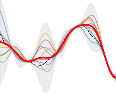
This figure shows 10 function draws from the posterior distribution using the above algorithm. The red line is the mean prediciton; the grey region represents the 3 standard deviations from 1,000 posterior draws; and the colored lines represent the 10 draws from the posterior.

Running the GP

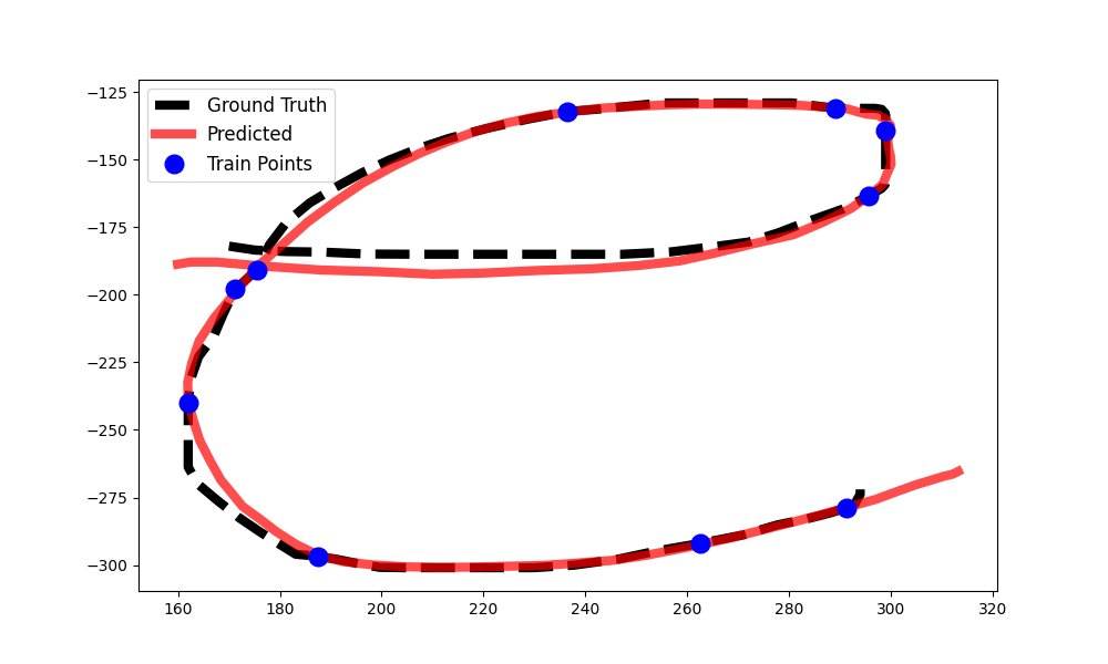
Putting it all together, we will apply the methods above to predict the \(X\) and \(Y\) trajectories of a randomly selected hand-drawn letter e in the data set, given only 10 randomly observed points along the time domain. In each scenario (for both dimensions), three kernels are used and their parameters are optimized. The kernel that produces the lowest negative log likelihood (or highest likelihood) will be used to plot the final trajectory prediction for the letter e. The main code for doing so is provided below.

import requests
import io

response = requests.get('https://www.drolet.io/projects/e_data.npy')
# Load trajectories, Shape: [N (num trajectories) X 100 (num samples) X 2 (num dimensions)]
e_data = np.load(io.BytesIO(response.content))

# Extract a random trajectory for testing
test_idx = np.random.choice(len(e_data))
print('Using test idx:', test_idx)
test_traj = e_data[test_idx]

# Use non-test data solely for fitting the scalers
scale_data = np.delete(e_data, [test_idx], axis=0)
x_scale = StandardScaler().fit(scale_data[:,:,0])
y_scale = StandardScaler().fit(scale_data[:,:,1])

num_train_points = 10  # Number of points to condition on (training points)
domain_ends = (0, 100)

# Define domain and randomly select points on the domain for the test trajectory
domain = np.linspace(domain_ends[0], domain_ends[1], e_data.shape[1])
domain_idxs = sorted(np.random.choice(range(e_data.shape[1]), 
                     num_train_points, replace=False))
T_obs = domain[domain_idxs]

# Get corresponding X trajectory values
obs, obs_full = dict(), dict()
obs_full['X_dim'] = x_scale.transform(e_data[test_idx,:,0].reshape(1,-1)).flat
obs['X_dim'] = obs_full['X_dim'][domain_idxs]

# Get corresponding Y trajectory values
obs_full['Y_dim'] = y_scale.transform(e_data[test_idx,:,1].reshape(1,-1)).flat
obs['Y_dim'] = obs_full['Y_dim'][domain_idxs]

# Define the lengthscale default to 1/10 of the domain length
lengthscale = Hyperparam(value=0.1*len(T_obs), bounds=[EPSILON, len(domain)/2])

##### Create the GaussianProcess Instances #####
GPs = {
    'X_dim' : {
        'SE' : GaussianProcess(kernel=SquaredExponential(lengthscale=lengthscale)),
        'RQ' : GaussianProcess(kernel=RationalQuadratic(lengthscale=lengthscale)),
        'Matern' : GaussianProcess(kernel=Matern(lengthscale=lengthscale))
    },
    'Y_dim' : {
        'SE' : GaussianProcess(kernel=SquaredExponential(lengthscale=lengthscale)),
        'RQ' : GaussianProcess(kernel=RationalQuadratic(lengthscale=lengthscale)),
        'Matern' : GaussianProcess(kernel=Matern(lengthscale=lengthscale))
    }
}

##### Perform Conditional Inference on data dimensions with the different kernels #####
for dim in GPs.keys():
    gp_dim = GPs[dim]
    for kernel in gp_dim.keys():
        gp = gp_dim[kernel]
        gp.data['X'], gp.data['f'] = T_obs.reshape(-1,1), obs[dim].reshape(-1,1)
        gp.nll = gp.optimize_kernel_hyperparams()
        gp.data['X*'] = domain.reshape(-1,1)
        gp.mu_post, gp.cov_post = gp.predict()
        gp.sim_draws = gp.simulate_posterior_draws(gp.mu_post, gp.cov_post, num_draws=1000)
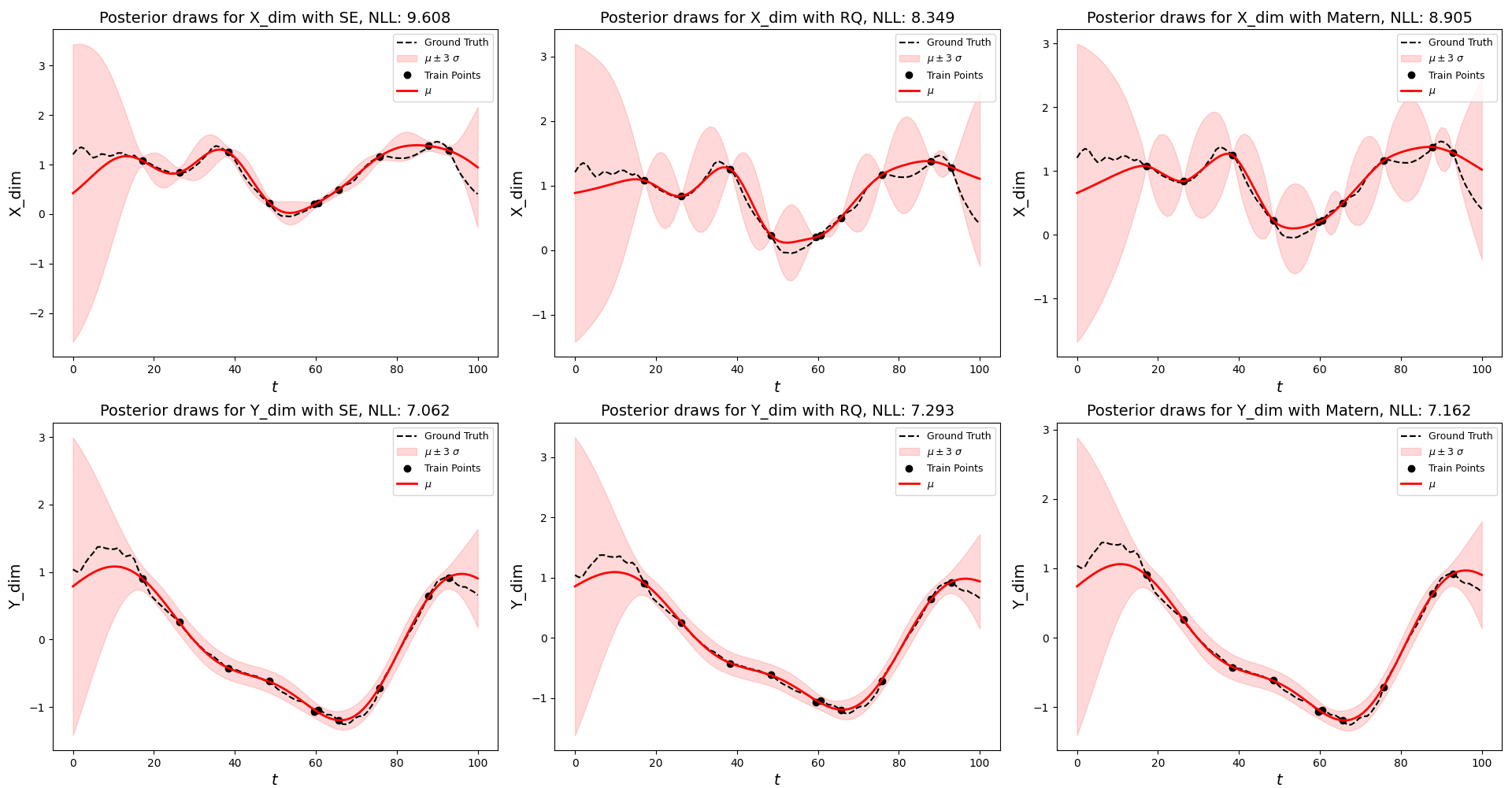

Top Figure: Conditional Posterior for Individual Trajectories with Different Kernels
Bottom Figure: Conditional Posterior Means for Lowest Negative Log Likelihood (NLL) Kernels Combined

The inference results for one of randomly selected examples is displayed above. It can be seen that different kernels produce different credible band regions and likelihood values. In some examples, the differences between kernel predictions are greatly exacerbated by the roughness of the trajectory or outlier test trajectories, but often times the different kernels produce similar looking results when the optimizer converges to sensible parameter values. I hope you enjoyed this walkthrough of Gaussian Process Prediction on hand-drawn trajectories! You can download the code for this demo here.

Appendix

Kernel and Hyperparameter Classes
# Define Hyperparameter Class
class Hyperparam:
    def __init__(self, value = 1.0, bounds = [-np.inf, np.inf]):
        self.value: float = value
        self.bounds : list = bounds

# Define Kernel Base Class
class Kernel():
    def __init__(self, hyperparams):
        self.hyperparams = dict()
        self.initialize_hyperparams(hyperparams)

    def get_hyperparam_names(self):
        return sorted(self.hyperparams.keys())

    def initialize_hyperparams(self, hyperparams: Dict[str, Hyperparam]):
        # Initialize the default hyperparam values and bounds
        defaults = {
            'alpha' : Hyperparam(value = 1.0, bounds = [EPSILON, 5.0]),
            'lengthscale' : Hyperparam(value = 10, bounds = [EPSILON, 50.0]),
            'sigma_f' : Hyperparam(value = 0.7, bounds = [EPSILON, 2.0]),
            'nu' : Hyperparam(value = 30, bounds = [EPSILON, 50.0])
        }

        # Fill in the hyperparams with defaults (if necessary)
        for hp_name in hyperparams.keys():
            hp = hyperparams[hp_name]
            self.hyperparams[hp_name] = Hyperparam()
            if hp:
                self.hyperparams[hp_name].value = defaults[hp_name].value if \
                                                  hp.value is None else hp.value
                self.hyperparams[hp_name].bounds = defaults[hp_name].bounds if \
                                                   hp.bounds is None else hp.bounds
            else:
                self.hyperparams[hp_name] = copy.deepcopy(defaults[hp_name])
Plotting Conditional Posterior
import matplotlib.pyplot as plt

##### Plot the Conditional Posterior #####
n_std = 3
fig, axs = plt.subplots(nrows=2, ncols=3, figsize=(16, 10))

# Iterate over all GPs and find the best ones
best_kernels = { 'X_dim' : None, 'Y_dim' : None }
for i, dim in enumerate(GPs.keys()):
    gp_dim = GPs[dim]
    best_nll = np.inf
    for j, kernel in enumerate(gp_dim.keys()):
        # Find best GP for given dim
        gp = gp_dim[kernel]
        if gp.nll < best_nll:
            best_kernels[dim] = kernel
            best_nll = gp.nll

        # Plot ground truth
        ax = axs[i,j]
        ax.plot(domain, obs_full[dim], 'k--', label='Ground Truth')
        # Plot mean +/- N Std Devs
        std = np.std(gp.sim_draws, axis=1)
        ax.fill_between(domain, gp.mu_post.flat-n_std*std, 
                        gp.mu_post.flat+n_std*std, color='red', alpha=0.15, 
                        label='$\mu \pm$' + str(n_std) + ' $\sigma$')
        # Plot the training points
        ax.plot(T_obs, obs[dim], 'ko', linewidth=2, label='Train Points')
        # Plot the mean of the posterior
        ax.plot(domain, gp.mu_post, 'r-', lw=2, label='$\mu$')
        
        # Add plot descriptions
        ax.set_xlabel('$t$', fontsize=14)
        ax.set_ylabel(dim, fontsize=14)
        ax.set_title('Posterior draws for ' + dim + ' with ' + kernel + 
                     ', NLL: ' + str(round(gp.nll, 3)), fontsize=14)
        ax.legend(fontsize=9)
plt.show()

##### Plot the Predicted Letter #####
# Get the "best" GPs according to NLL values
gp_x, gp_y = GPs['X_dim'][best_kernels['X_dim']], GPs['Y_dim'][best_kernels['Y_dim']]
fig, ax = plt.subplots(nrows=1, ncols=1, figsize=(10, 6))
# Plot original trajectory
x_data, y_data = e_data[test_idx,:,0].flat, e_data[test_idx,:,1].flat
ax.plot(x_data, y_data, 'k--', label='Ground Truth', lw=6)

# Plot the mean predicted trajectory
mu_x = x_scale.inverse_transform(gp_x.mu_post.reshape(1,-1)).flat
mu_y = y_scale.inverse_transform(gp_y.mu_post.reshape(1,-1)).flat
ax.plot(mu_x, mu_y, color='r', label='Predicted', lw=6, alpha=0.7)
ax.plot(x_data[domain_idxs], y_data[domain_idxs], 'bo', 
        label='Train Points', markersize=12)
ax.legend(fontsize=12)
plt.show()

References

  1. The Kernel Cookbook: https://www.cs.toronto.edu/~duvenaud/cookbook/ 

  2. Rasmussen, Carl Edward, and Christopher K. I. Williams. Gaussian Processes for Machine Learning. MIT Press, 2005. https://gaussianprocess.org/gpml/  2

Gaussian Process Prediction

GP Regression on Hand-Drawn Trajectories

Gaussian Process (GP) Regression is a powerful tool for performing inference on sparse data, such as in situations where the whole trajectory cannot be observed or it is impractical to do so. For example, if we are trying to quantify the mineral content in a spatial field- where only a finite number of samples are to be collected- then the values at unknown locations can be predicted using a closely-related method known as kriging. Consider being given a data set which cointains a few points along a trajectory, and the goal is to infer what the whole trajectory looks like. If you have prior knowledge on the behavior of the function in between regression points, a covariance function (kernel) can be chosen, acting as a prior on the distribution of functions that the true process is sampled from (although choosing a kernel is not always straightforward). Upon observing new data points, conditional inference allows for combining the existing (prior) estimate and the newly observed data to obtain a new (posterior) estimate of the underlying function. This iterative procedure is convenient for updating our belief of the true trajectory as data comes sequentially, but often the conditional inference step only needs to be applied once (in the event where all of the data points are provided at once, as in the upcoming example).

GP Regression is a compelling option for nonlinear regression since it can be used to quantify the uncertainty of values in between observed points (with credible bands) and provides a flexible way to incorporate a prior with covariance functions. Moreover, the kernel hyperparameters can be estimated by maximizing the marginal likelihood of the training points given their domain locations, and this post will describe the process for doing so. With the popularity of neural networks, an obvious question is whether a neural network can be used for the prediction instead. I did a project on this with a peer, where both methods were used to predict a hand-drawn trajectory of the letter e, and both methods predicted the full trajectory well. I’m not an expert in this area, but I wouldn’t be surprised if there are good ways to approximate the credible bands using NNs (e.g., with stochastic forward passes), but that’s beyond the scope of this post. Overall, there are some cool features in GP Regression that a vanilla, feed-forward NN does not provide out of the box. Let’s check it out!

The Hand-Drawn Data Set

The following data set (left) was created using a computer mouse and python script to record the cursor positions on the canvas from drawing the letter e. All demonstrations are resampled to have the same length. These trajectories can be used by extracting the \(x\) and \(y\) dimensions to fit two Gaussian Processes independently.

Distribution of hand-drawn letter e's
Distribution of X (top) and Y (bottom) Coordinates from start to finish (not standardized)

Choosing the Kernel

As noted above, different kernels can be chosen based on the data points observed in the sample set. Looking at the trajectories for the \(X\) and \(Y\) components of the letter e, we can see that they exhibits smooth (almost sinusoidal) behavior. Knowing this, the Squared Exponential (SE) kernel becomes a good candidate since it is often used for fitting smooth functions. Other popular kernels for fitting Gaussian Processes include the Rational Quadratic (RQ) and Matern kernel, which is grounded with many theoretical properties. We will use all three of these kernels and compare their marginal likelihoods to determine which one to use. The respective definitions for these kernels are listed below.

$$ k(x_i, x_j) = \sigma_f^2 \exp{ \left( -\frac{(x_i- x_j)^2}{2\ell^2} \right)} $$
Squared Exponential Kernel
$$ k(x_i, x_j) = \sigma_f^2 \left( 1 + \frac{(x_i - x_j)^2}{2 \alpha \ell^2} \right)^{-\alpha} $$
Rational Quadratic Kernel
$$ k(x_i, x_j) = \frac{2^{1-\nu}}{\Gamma(\nu)}\Bigg( \frac{\sqrt{2\nu} \lVert x_i - x_j \rVert }{\ell} \Bigg)^\nu K_\nu\Bigg( \frac{\sqrt{2\nu} \lVert x_i - x_j \rVert }{\ell} \Bigg) $$
Matern Kernel

The following code implements the kernels above by inheriting from a Kernel base class (see Appendix), and the mathematical defintions are specified in the cov method. Included in each class are the respective kernel hyperparameters which later optimized. The Kernel instance is passed to the Gaussian Process class for prediction in the upcoming section. The cdist function from scipy is a computationally efficient way to compute the distance between pairs of points compared to naive \(O(n^2)\) implementation using for loops. For more information on kernels, check out the references and The Kernel Cookbook 1.

from scipy.spatial.distance import cdist
from scipy.special import gamma, kv

EPSILON = 1e-8

# Define the SE Kernel
class SquaredExponential(Kernel):
    def __init__(self, sigma_f: Hyperparam = None, lengthscale: Hyperparam = None):
        _hyperparams = {
            'sigma_f' : sigma_f,
            'lengthscale' : lengthscale,
        }
        super().__init__(_hyperparams)

    # Covariance function definition
    def cov(self, xi, xj):
        sf, l = self.hyperparams['sigma_f'], self.hyperparams['lengthscale']
        dist = cdist(xi, xj, 'sqeuclidean') 
        covariance = sf**2 * np.exp(-dist/(2*l**2))
        return covariance

# Define the RQ Kernel
class RationalQuadratic(Kernel):
    def __init__(self, sigma_f: Hyperparam = None, 
                 lengthscale: Hyperparam = None, alpha: Hyperparam = None):
        _hyperparams = {
            'sigma_f' : sigma_f,
            'lengthscale' : lengthscale,
            'alpha' : alpha
        }
        super().__init__(_hyperparams)
    
    # Covariance function definition
    def cov(self, xi, xj):
        sf, l, a = self.hyperparams['sigma_f'], self.hyperparams['lengthscale'], \
                   self.hyperparams['alpha']
        dist = cdist(xi, xj, 'sqeuclidean')
        covariance = sf**2 * (1 + dist/(2*a * l**2))**(-a)
        return covariance

# Define the Matern Kernel
class Matern(Kernel):
    def __init__(self, nu: Hyperparam = None, lengthscale: Hyperparam = None):
        _hyperparams = {
            'nu' : nu,
            'lengthscale' : lengthscale,
        }
        super().__init__(_hyperparams)

    # Covariance function definition
    def cov(self, xi, xj):
        v, l = self.hyperparams['nu'], self.hyperparams['lengthscale']
        coeff = (2 ** (1 - v)) / gamma(v)
        dist = cdist(xi, xj, 'euclidean')
        dist[dist == 0] = EPSILON
        dist *= (np.sqrt(2 * v) / l)
        covariance = coeff * dist**v * kv(v, dist)
        return covariance


Performing Inference

Inference for the conditional posterior is given by the standard set of equations for the joint Gaussian distribution. For this post, I use the notation from Rasmussen’s Gaussian Processes for Machine Learning book 2, which is a great and comprehensive overview of this topic. The code in the upcoming section also adheres to this notation. Overall, the joint distribution of the training points and prediction points are given as follows (where the *’s denote predictions). We let \(\mathbf{y} = \mathbf{f}(\mathbf{x}) + \epsilon\) represent the noisy observations by including an additive noise term, which simply reduces to \(\mathbf{y} = \mathbf{f(x)} = \mathbf{f}\) in the absense of noise. However, the noise term \(\sigma_n\) is included in the marginal likelihood optimization, having a starting value of \(0\) when passed to the optimizer. This gives us the following equations:

\[\begin{equation*} \begin{split} \mathbf{f_*} \mid X_*, X, \mathbf{y} \sim \mathcal{N} & \left( K(X_*, X)[K(X,X) + \sigma_n^2I]^{-1}\mathbf{y}, \right. \\ & \hspace{-10mm} \left. K(X_*,X_*) - K(X_*, X)[K(X,X) + \sigma_n^2]^{-1} K(X, X_*) \right) \end{split} \end{equation*}\]

with the joint distribution being defined as,

\[\begin{bmatrix} \mathbf{y} \\ \mathbf{f_*} \\ \end{bmatrix} \sim \mathcal{N}\left( \mathbf{0}, \begin{bmatrix} K(X, X) + \sigma_n^2I & K(X, X_*) \\ K(X*, X) & K(X*, X_*) \\ \end{bmatrix} \right)\]

Unless a mean function is specified (e.g, through Radial Basis Functions), the Gaussian Process is typically implemented with a zero-mean assumption. In this example, we coerce the trajectories into a zero-mean distribution using standardization, which is seemingly appropriate given the distribution of the \(X\) and \(Y\) trajectories displayed in the first figure; however, this may not always be appropriate. Conditional inference lies at the heart of Gaussian Process Regression, and the algorithm for doing so- as well as for estimating the hyperparameters by maximizing the marginal likelihood- is described in Algorithm 2.1 in Rasmussen 2. This algorithm is re-iterated below.

Algorithm 2.1 (Rasmussen) : Log Marginal Likelihood using the Cholesky factorization $$ \begin{align*} L &:= \text{cholesky}(K + \sigma_n^2I) \\ \mathbf{\alpha} &:= L^{\top} \backslash \left(L \backslash \mathbf{y} \right) \\ \bar{\mathcal{f}_*} &:= \mathbf{k_*}^{\top} \mathbf{\alpha} \\ \mathbf{v} &:= L \backslash \mathbf{k_*} \\ \mathbb{V}[\mathcal{f_*}] &:= k(\mathbf{x_*, x_*}) - \mathbf{v}^{\top}\mathbf{v} \\ \log p(\mathbf{y} \mid X) &:= -\frac{1}{2}\mathbf{y}^{\top}\mathbf{\alpha} - \sum_i \log L_{ii} - \frac{n}{2}\log 2\pi \end{align*} $$

This algorithm is implemented below in the predict method of the GaussianProcess class, however, the negative log-likelihood is computed instead since it will be minimized. The constant term, \(-\frac{n}{2}\log 2 \pi\), is also omitted since it does not affect the optimization of the hyperparameters. The Cholesky factorization is convenient for inverting matrices since it is faster, more numerically stable, and provides a convenient way to sample from the posterior. Clearly this factorization is used in Algorithm 2.1 to compute the conditional posterior as opposed to inverting the \(K(X, X) + \sigma_n^2 I\) term in the preceding equations. The code below was written to resemble the posterior mean and covariance computations in Algorithm 2.1. Notably, there are some redundant calculations (i.e, the covariance computations, which is not a big factor when using a small number of training points), but this is simply for readability purposes.

# Define Gaussian Process Class
from numpy.linalg import solve, cholesky
from scipy.optimize import minimize

class GaussianProcess():
    def __init__(self, kernel: Kernel):
        self.kernel = kernel
        self.sigma_n = Hyperparam(value=0.0, bounds=[EPSILON, 3])
        # Initialize data struct to store train/test points
        self.data = {
            'X' : np.array([]),
            'f' : np.array([]),
            'X*' : np.array([])
        }

    # Notational wrapper for the Kernel
    def _K(self, XiXj: str):
        Xi, Xj = str.split(XiXj,', ')
        cov = self.kernel.cov(self.data[Xi], self.data[Xj])
        return cov

    # Calculate conditional posterior (Rasmussen)
    # NOTE: there are redundant computations (strictly for readability)
    def predict(self):
        K, f, n = self._K, self.data['f'], len(self.data['X'])
        L = cholesky(K('X, X') + np.eye(n)*self.sigma_n.value**2)
        alpha = solve(L.T, solve(L, f))
        mu_post = K('X, X*').T @ alpha
        v = solve(L, K('X, X*'))
        cov_post = K('X*, X*') - (v.T @ v)
        return (mu_post, cov_post)


Likelihood Optimization:

As mentioned, the marginal likelihood is used to optimize the kernel hyperparameters before performing predictions. The naive way of computing the likelihood (by marginalizing over the function values \(\mathbf{f}\)) is given by:

\[\log p(\mathbf{y} \, | \, X, \theta) =- \frac{1}{2} \mathbf{y}^{\top} K_y(\theta)^{-1} \mathbf{y} - \frac{1}{2} \log |K_y(\theta)| - \frac{n}{2} \log 2\pi.\]

Using the Cholesky decomposition (as in Algorithm 2.1), we get the following equivalent expression. This function below is the objective function used with scipy’s minimize function.

\[\log p(\mathbf{y} \, | \, X ,\theta) = -\frac{1}{2} \, \mathbf{y}^{\top} \mathbf{\alpha} \; - \sum \log L_{ii} - \frac{n}{2} \, \log 2\pi\]
    # Negative Log-Likelihood for Kernel Hyperparameters
    def _nll_kernel_hyperparams(self, hyperparam_values):
        K, f, n = self._K, self.data['f'], len(self.data['X'])
        # Set the kernel parameters to the input from the optimizer
        for name, value in zip(self.kernel.get_hyperparam_names(), hyperparam_values):
            self.kernel.hyperparams[name] = value
        self.sigma_n.value = hyperparam_values[-1]
        
        # If the proposed optimizer values cause the matrix to be non-PSD, return inf
        try: L = cholesky(K('X, X') + np.eye(n)*self.sigma_n.value**2) 
        except: return np.inf
        
        alpha = solve(L.T, solve(L, f))
        loglik = -0.5*(f.T @ alpha) - np.trace(L)
        return -loglik
    
    def optimize_kernel_hyperparams(self):
        # Initialize the starting values for the hyperparams
        starting_vals = [self.kernel.hyperparams[name].value \
                         for name in self.kernel.get_hyperparam_names()]
        starting_vals.append(self.sigma_n.value) # append the sigma_n term
        
        # Set the bounds for the hyperparams
        hp_bounds = [self.kernel.hyperparams[name].bounds \
                     for name in self.kernel.get_hyperparam_names()]
        hp_bounds.append(self.sigma_n.bounds)
        
        # Minimize the marginal likelihood
        cost = minimize(self._nll_kernel_hyperparams, starting_vals, 
                        bounds=hp_bounds, method='L-BFGS-B')
        nll = cost.fun
        print('Optimized values for kernel hyperparameters (NLL = ' + str(nll) + \ 
              ') :\n', self.kernel.hyperparams, end=" ")
        print(', sigma_n: ', self.sigma_n.value)
        return nll


Without the hyperparameter bounds (above), the optimizer may propose negative values for the \(\sigma\) terms or large values to the exponent terms (e.g., the \(\alpha\) term for the Rational Quadratic kernel), causing numerical instability such that posterior samples cannot be drawn. After optimizing the hyperparameters for the three different kernels described above, samples are drawn from the posterior. The Cholesky decomposition is used to sample from the posterior. A small ridge term (\(\epsilon\)) is added to the diagonal of the covariance matrix to improve stability.

Drawing from Posterior

    def simulate_posterior_draws(self, mu_post, cov_post, num_draws):
        L_post = cholesky(cov_post + np.eye(cov_post.shape[1])*EPSILON)
        sim_draws = mu_post + L_post @ np.random.normal(size=(L_post.shape[1], num_draws))
        return sim_draws
This figure shows 10 function draws from the posterior distribution using the above algorithm. The red line is the mean prediciton; the grey region represents the 3 standard deviations from 1,000 posterior draws; and the colored lines represent the 10 draws from the posterior.

Running the GP

Putting it all together, we will apply the methods above to predict the \(X\) and \(Y\) trajectories of a randomly selected hand-drawn letter e in the data set, given only 10 randomly observed points along the time domain. In each scenario (for both dimensions), three kernels are used and their parameters are optimized. The kernel that produces the lowest negative log likelihood (or highest likelihood) will be used to plot the final trajectory prediction for the letter e. The main code for doing so is provided below.

import requests
import io

response = requests.get('https://www.drolet.io/projects/e_data.npy')
# Load trajectories, Shape: [N (num trajectories) X 100 (num samples) X 2 (num dimensions)]
e_data = np.load(io.BytesIO(response.content))

# Extract a random trajectory for testing
test_idx = np.random.choice(len(e_data))
print('Using test idx:', test_idx)
test_traj = e_data[test_idx]

# Use non-test data solely for fitting the scalers
scale_data = np.delete(e_data, [test_idx], axis=0)
x_scale = StandardScaler().fit(scale_data[:,:,0])
y_scale = StandardScaler().fit(scale_data[:,:,1])

num_train_points = 10  # Number of points to condition on (training points)
domain_ends = (0, 100)

# Define domain and randomly select points on the domain for the test trajectory
domain = np.linspace(domain_ends[0], domain_ends[1], e_data.shape[1])
domain_idxs = sorted(np.random.choice(range(e_data.shape[1]), 
                     num_train_points, replace=False))
T_obs = domain[domain_idxs]

# Get corresponding X trajectory values
obs, obs_full = dict(), dict()
obs_full['X_dim'] = x_scale.transform(e_data[test_idx,:,0].reshape(1,-1)).flat
obs['X_dim'] = obs_full['X_dim'][domain_idxs]

# Get corresponding Y trajectory values
obs_full['Y_dim'] = y_scale.transform(e_data[test_idx,:,1].reshape(1,-1)).flat
obs['Y_dim'] = obs_full['Y_dim'][domain_idxs]

# Define the lengthscale default to 1/10 of the domain length
lengthscale = Hyperparam(value=0.1*len(T_obs), bounds=[EPSILON, len(domain)/2])

##### Create the GaussianProcess Instances #####
GPs = {
    'X_dim' : {
        'SE' : GaussianProcess(kernel=SquaredExponential(lengthscale=lengthscale)),
        'RQ' : GaussianProcess(kernel=RationalQuadratic(lengthscale=lengthscale)),
        'Matern' : GaussianProcess(kernel=Matern(lengthscale=lengthscale))
    },
    'Y_dim' : {
        'SE' : GaussianProcess(kernel=SquaredExponential(lengthscale=lengthscale)),
        'RQ' : GaussianProcess(kernel=RationalQuadratic(lengthscale=lengthscale)),
        'Matern' : GaussianProcess(kernel=Matern(lengthscale=lengthscale))
    }
}

##### Perform Conditional Inference on data dimensions with the different kernels #####
for dim in GPs.keys():
    gp_dim = GPs[dim]
    for kernel in gp_dim.keys():
        gp = gp_dim[kernel]
        gp.data['X'], gp.data['f'] = T_obs.reshape(-1,1), obs[dim].reshape(-1,1)
        gp.nll = gp.optimize_kernel_hyperparams()
        gp.data['X*'] = domain.reshape(-1,1)
        gp.mu_post, gp.cov_post = gp.predict()
        gp.sim_draws = gp.simulate_posterior_draws(gp.mu_post, gp.cov_post, num_draws=1000)

Top Figure: Conditional Posterior for Individual Trajectories with Different Kernels
Bottom Figure: Conditional Posterior Means for Lowest Negative Log Likelihood (NLL) Kernels Combined

The inference results for one of randomly selected examples is displayed above. It can be seen that different kernels produce different credible band regions and likelihood values. In some examples, the differences between kernel predictions are greatly exacerbated by the roughness of the trajectory or outlier test trajectories, but often times the different kernels produce similar looking results when the optimizer converges to sensible parameter values. I hope you enjoyed this walkthrough of Gaussian Process Prediction on hand-drawn trajectories! You can download the code for this demo here.

Appendix

Kernel and Hyperparameter Classes
# Define Hyperparameter Class
class Hyperparam:
    def __init__(self, value = 1.0, bounds = [-np.inf, np.inf]):
        self.value: float = value
        self.bounds : list = bounds

# Define Kernel Base Class
class Kernel():
    def __init__(self, hyperparams):
        self.hyperparams = dict()
        self.initialize_hyperparams(hyperparams)

    def get_hyperparam_names(self):
        return sorted(self.hyperparams.keys())

    def initialize_hyperparams(self, hyperparams: Dict[str, Hyperparam]):
        # Initialize the default hyperparam values and bounds
        defaults = {
            'alpha' : Hyperparam(value = 1.0, bounds = [EPSILON, 5.0]),
            'lengthscale' : Hyperparam(value = 10, bounds = [EPSILON, 50.0]),
            'sigma_f' : Hyperparam(value = 0.7, bounds = [EPSILON, 2.0]),
            'nu' : Hyperparam(value = 30, bounds = [EPSILON, 50.0])
        }

        # Fill in the hyperparams with defaults (if necessary)
        for hp_name in hyperparams.keys():
            hp = hyperparams[hp_name]
            self.hyperparams[hp_name] = Hyperparam()
            if hp:
                self.hyperparams[hp_name].value = defaults[hp_name].value if \
                                                  hp.value is None else hp.value
                self.hyperparams[hp_name].bounds = defaults[hp_name].bounds if \
                                                   hp.bounds is None else hp.bounds
            else:
                self.hyperparams[hp_name] = copy.deepcopy(defaults[hp_name])
Plotting Conditional Posterior
import matplotlib.pyplot as plt

##### Plot the Conditional Posterior #####
n_std = 3
fig, axs = plt.subplots(nrows=2, ncols=3, figsize=(16, 10))

# Iterate over all GPs and find the best ones
best_kernels = { 'X_dim' : None, 'Y_dim' : None }
for i, dim in enumerate(GPs.keys()):
    gp_dim = GPs[dim]
    best_nll = np.inf
    for j, kernel in enumerate(gp_dim.keys()):
        # Find best GP for given dim
        gp = gp_dim[kernel]
        if gp.nll < best_nll:
            best_kernels[dim] = kernel
            best_nll = gp.nll

        # Plot ground truth
        ax = axs[i,j]
        ax.plot(domain, obs_full[dim], 'k--', label='Ground Truth')
        # Plot mean +/- N Std Devs
        std = np.std(gp.sim_draws, axis=1)
        ax.fill_between(domain, gp.mu_post.flat-n_std*std, 
                        gp.mu_post.flat+n_std*std, color='red', alpha=0.15, 
                        label='$\mu \pm$' + str(n_std) + ' $\sigma$')
        # Plot the training points
        ax.plot(T_obs, obs[dim], 'ko', linewidth=2, label='Train Points')
        # Plot the mean of the posterior
        ax.plot(domain, gp.mu_post, 'r-', lw=2, label='$\mu$')
        
        # Add plot descriptions
        ax.set_xlabel('$t$', fontsize=14)
        ax.set_ylabel(dim, fontsize=14)
        ax.set_title('Posterior draws for ' + dim + ' with ' + kernel + 
                     ', NLL: ' + str(round(gp.nll, 3)), fontsize=14)
        ax.legend(fontsize=9)
plt.show()

##### Plot the Predicted Letter #####
# Get the "best" GPs according to NLL values
gp_x, gp_y = GPs['X_dim'][best_kernels['X_dim']], GPs['Y_dim'][best_kernels['Y_dim']]
fig, ax = plt.subplots(nrows=1, ncols=1, figsize=(10, 6))
# Plot original trajectory
x_data, y_data = e_data[test_idx,:,0].flat, e_data[test_idx,:,1].flat
ax.plot(x_data, y_data, 'k--', label='Ground Truth', lw=6)

# Plot the mean predicted trajectory
mu_x = x_scale.inverse_transform(gp_x.mu_post.reshape(1,-1)).flat
mu_y = y_scale.inverse_transform(gp_y.mu_post.reshape(1,-1)).flat
ax.plot(mu_x, mu_y, color='r', label='Predicted', lw=6, alpha=0.7)
ax.plot(x_data[domain_idxs], y_data[domain_idxs], 'bo', 
        label='Train Points', markersize=12)
ax.legend(fontsize=12)
plt.show()

References

  1. The Kernel Cookbook: https://www.cs.toronto.edu/~duvenaud/cookbook/ 

  2. Rasmussen, Carl Edward, and Christopher K. I. Williams. Gaussian Processes for Machine Learning. MIT Press, 2005. https://gaussianprocess.org/gpml/  2